
Simulating a BPX parameter set and comparing with its validation data
BPX (Battery Parameter eXchange) is an open standard for physics-based battery parameter sets. Besides the parameters and the operating conditions of the cell, a BPX file can contain validation data: measured or simulated curves that the parameter set is expected to reproduce.
In this example we
load the BPX parameterisation of an NMC111|graphite 12.5 Ah pouch cell,
simulate a discharge within the BPX operating conditions,
simulate the experiments of the
Validationsection and compare them with the data, andwrite the parameter set back to a BPX file.
See BPX parameter sets for a description of the conversion.
using BattMo, GLMakieLoad the cell parameters
load_cell_parameters converts the BPX parameters to BattMo cell parameters. The conversion is summarised in one warning, with everything that differs from the BPX input or needs attention, and one info message with the details. For this file, the warning reports that the OCPs give 4.2018 V at the stoichiometry limits, slightly above the upper cut-off voltage of 4.2 V, and that BattMo does not use the lumped thermal model of BPX, which does not matter for the isothermal simulations below.
bpx_file_path = joinpath(dirname(pathof(BattMo)), "..", "test", "data", "jsonfiles", "nmc_pouch_cell_BPX.json")

cell_parameters = load_cell_parameters(; from_bpx_file_path = bpx_file_path)
{
"Electrolyte" => {
"TransferenceNumber" => 0.2594
"SpecificHeatCapacity" => 913
"Concentration" => 1000
"IonicConductivity" => "(0.1297 * (c / 1000) ^ 3 - 2.51 * (c / 1000) ^ 1.5 + 3.329 * (c / 1000)) * exp(17100 / 8.31446261815324 * (1.0 / 298.15 - 1.0 / T))"
"ChargeNumber" => 1
"DiffusionCoefficient" => "(8.794e-11 * (c / 1000) ^ 2 - 3.972e-10 * (c / 1000) + 4.862e-10) * exp(17100 / 8.31446261815324 * (1.0 / 298.15 - 1.0 / T))"
"Density" => 1847
"ThermalConductivity" => 2.04
"BruggemanCoefficient" => {
"PositiveElectrode" => 1.4998754833259478
"NegativeElectrode" => 1.500029440241825
"Separator" => 1.500064808421937
}
}
"PositiveElectrode" => {
"Coating" => {
"EffectiveDensity" => 1334.470429
"Thickness" => 5.23e-5
"BruggemanCoefficient" => 1.4998754833259478
}
"ConductiveAdditive" => {
"Description" => "Not provided by BPX; zero-mass placeholder."
"ThermalConductivity" => 2.04
"SpecificHeatCapacity" => 913
"MassFraction" => 0.0
"Density" => 1847
"ElectronicConductivity" => 1.2846840673435724
}
"Binder" => {
"Description" => "Not provided by BPX; lumps all inactive solid (binder and conductive additive)."
"ThermalConductivity" => 2.04
"SpecificHeatCapacity" => 913
"MassFraction" => 0.08303947228192943
"Density" => 1847
"ElectronicConductivity" => 1.2846840673435724
}
"ActiveMaterial" => {
"ThermalConductivity" => 2.04
"ChargeTransferCoefficient" => 0.5
"MassFraction" => 0.9169605277180706
"VolumetricSurfaceArea" => 432072
"Density" => 1847
"StoichiometricCoefficientAtSOC100" => 0.42424
"NumberOfElectronsTransfered" => 1
"ReactionRateConstant" => 1.5777164516640942e-11
"ParticleRadius" => 4.6e-6
"ActivationEnergyOfReaction" => 35000
"SpecificHeatCapacity" => 913
"StoichiometricCoefficientAtSOC0" => 0.9621
"OpenCircuitPotential" => "-3.04420906 * (c / cmax) + 10.04892207 - 0.65637536 * tanh(-4.02134095 * ((c / cmax) - 0.80063948)) + 4.24678547 * tanh(12.17805062 * ((c / cmax) - 7.57659337)) - 0.3757068 * tanh(59.33067782 * ((c / cmax) - 0.99784492))"
"DiffusionCoefficient" => 3.2e-14
"ElectronicConductivity" => 1.2846840673435724
"ActivationEnergyOfDiffusion" => 15000
"EntropyChange" => -0.0001
"MaximumConcentration" => 46200
}
}
"Cell" => {
"NumberOfLayersInParallel" => 34
"ReferenceTemperature" => 298.15
"ElectrodeGeometricSurfaceArea" => 0.016808
"Case" => "Pouch"
"NominalCapacity" => 12.5
"DeviceSurfaceArea" => 0.0379
"DoubleCoatedElectrodes" => false
}
"Metadata" => {
"Description" => "NMC111|graphite 12.5 Ah pouch cell. Parameterisation by About:Energy Limited (aboutenergy.io), December 2022, based on cell cycling data, and electrode data gathered after cell teardown. Electrolyte properties from Nyman et al. 2008 (doi:10.1016/j.electacta.2008.04.023). Negative electrode entropic coefficient data are from O'Regan et al. 2022 (doi:10.1016/j.electacta.2022.140700). Positive electrode entropic coefficient data are from Viswanathan et al. 2010 (doi:10.1016/j.jpowsour.2009.11.103). Other thermal properties are estimated."
"Title" => "Parameterisation example of an NMC111|graphite 12.5 Ah pouch cell"
"Models" => {
"ModelFramework" => "P2D"
"TransportInSolid" => "FullDiffusion"
}
"Source" => "Converted from a BPX 1.1.1 parameter set"
}
"NegativeElectrode" => {
"Coating" => {
"EffectiveDensity" => 1377.8786229999998
"Thickness" => 5.62e-5
"BruggemanCoefficient" => 1.500029440241825
}
"ConductiveAdditive" => {
"Description" => "Not provided by BPX; zero-mass placeholder."
"ThermalConductivity" => 2.04
"SpecificHeatCapacity" => 913
"MassFraction" => 0.0
"Density" => 1847
"ElectronicConductivity" => 0.34454077043552944
}
"Binder" => {
"Description" => "Not provided by BPX; lumps all inactive solid (binder and conductive additive)."
"ThermalConductivity" => 2.04
"SpecificHeatCapacity" => 913
"MassFraction" => 0.08042635768022444
"Density" => 1847
"ElectronicConductivity" => 0.34454077043552944
}
"ActiveMaterial" => {
"ThermalConductivity" => 2.04
"ChargeTransferCoefficient" => 0.5
"MassFraction" => 0.9195736423197756
"VolumetricSurfaceArea" => 499522
"Density" => 1847
"StoichiometricCoefficientAtSOC100" => 0.75668
"NumberOfElectronsTransfered" => 1
"ReactionRateConstant" => 5.529997159507368e-12
"ParticleRadius" => 4.12e-6
"ActivationEnergyOfReaction" => 55000
"SpecificHeatCapacity" => 913
"StoichiometricCoefficientAtSOC0" => 0.005504
"OpenCircuitPotential" => "9.47057878e-01 * exp(-1.59418743e+02 * (c / cmax)) - 3.50928033e+04 + 1.64230269e-01 * tanh(-4.55509094e+01 * ((c / cmax) - 3.24116012e-02 )) + 3.69968491e-02 * tanh(-1.96718868e+01 * ((c / cmax) - 1.68334476e-01)) + 1.91517003e+04 * tanh(3.19648312e+00 * ((c / cmax) - 1.85139824e+00)) + 5.42448511e+04 * tanh(-3.19009848e+00 * ((c / cmax) - 2.01660395e+00))"
"DiffusionCoefficient" => 2.728e-14
"ElectronicConductivity" => 0.34454077043552944
"ActivationEnergyOfDiffusion" => 30000
"EntropyChange" => "(-0.1112 * (c / cmax) + 0.02914 + 0.3561 * exp(-(((c / cmax) - 0.08309) ^ 2) / 0.004616)) / 1000"
"MaximumConcentration" => 29730
}
}
"Separator" => {
"ThermalConductivity" => 2.04
"SpecificHeatCapacity" => 913
"Density" => 1847
"Thickness" => 2.0e-5
"BruggemanCoefficient" => 1.500064808421937
"Porosity" => 0.47
}
}The converted parameters can be inspected and modified in the usual way. The BPX cell consists of 34 electrode pairs of 168 cm², which BattMo represents as 34 single coated electrode layers.
cell = cell_parameters["Cell"]
println("Electrode area of one layer: ", cell["ElectrodeGeometricSurfaceArea"], " m²")
println("Number of layers:            ", cell["NumberOfLayersInParallel"])
println("Total electrode area:        ", compute_total_electrode_area(cell_parameters), " m²")
Electrode area of one layer: 0.016808 m²
Number of layers: 34
Total electrode area: 0.571472 m²Simulate a discharge within the BPX operating conditions
The operating conditions of the BPX file (voltage cut-offs, initial state of charge and temperatures) belong to the cycling protocol in BattMo. load_cycling_protocol reads them from the BPX file. BPX does not define a cycling experiment, so a constant current discharge with DRate = 1 is set up, which the warning points out.
cycling_protocol = load_cycling_protocol(; from_bpx_file_path = bpx_file_path){
"DRate" => 1.0
"LowerVoltageLimit" => 2.7
"AmbientTemperature" => 298.15
"Protocol" => "CC"
"Metadata" => {
"Description" => "Constant current discharge within the voltage window of the BPX parameter set."
"Title" => "Parameterisation example of an NMC111|graphite 12.5 Ah pouch cell"
"Source" => "Converted from BPX"
}
"UpperVoltageLimit" => 4.2
"InitialControl" => "discharging"
"InitialTemperature" => 298.15
"TotalNumberOfCycles" => 0
"InitialStateOfCharge" => 1
}The DRate is relative to the theoretical capacity that BattMo computes from the electrode parameters, not to the nominal capacity of the BPX file. For a discharge at the nominal 1C current of 12.5 A, we set the rate relative to the theoretical capacity.
capacity = compute_cell_theoretical_capacity(cell_parameters)
println("Nominal capacity:     ", cell["NominalCapacity"], " Ah")
println("Theoretical capacity: ", round(capacity, digits = 2), " Ah")

cycling_protocol["DRate"] = cell["NominalCapacity"] / capacity

model = LithiumIonBattery()
output = solve(Simulation(model, cell_parameters, cycling_protocol); info_level = -1)

plot_dashboard(output; plot_type = "simple")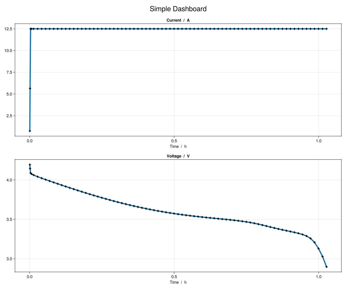
Simulate the validation experiments
The Validation section of this file contains a C/20 and a 1C discharge. With the experiment option, load_full_simulation_input sets up a complete simulation input in which the current of the chosen experiment is prescribed with the InputCurrentSeries protocol. The current is converted from the BPX sign convention (positive for charging) to the BattMo one (positive for discharging); the import checks that the sign of the current matches the voltage curve and the name of the experiment.
For each experiment we run the simulation and compute the root mean square error of the voltage. The simulation uses the times of the data as time steps, so the simulated and measured voltages are compared at the same times. The first output is at the end of the first time step, so the voltage at time zero is not compared.
experiments = ["C/20 discharge", "1C discharge"]
validation = BattMo.JSON.parsefile(bpx_file_path)["Validation"]

results = map(experiments) do experiment
    simulation_input = load_full_simulation_input(;
        from_bpx_file_path = bpx_file_path,
        bpx_options = (experiment = experiment,),
    )
    output = run_simulation(simulation_input; info_level = -1)

    time = output.time_series["Time"]
    voltage = output.time_series["Voltage"]

    data = validation[experiment]
    time_data = Float64.(data["Time [s]"])
    voltage_data = Float64.(data["Voltage [V]"])

    # Compare at the times of the data within the simulated time span
    compared = [findfirst(t -> isapprox(t, t_data), time) for t_data in time_data]
    measured = .!isnothing.(compared)
    error = voltage[compared[measured]] .- voltage_data[measured]
    rmse = sqrt(sum(error .^ 2) / length(error))
    println(rpad(experiment, 16), "RMSE ", round(1000 * rmse, digits = 1), " mV")

    (; experiment, time, voltage, time_data, voltage_data, rmse)
end
2-element Vector{@NamedTuple{experiment::String, time::Vector{Float64}, voltage::Vector{Float64}, time_data::Vector{Float64}, voltage_data::Vector{Float64}, rmse::Float64}}:
(experiment = "C/20 discharge", time = [1000.0, 2000.0, 3000.0, 4000.0, 5000.0, 6000.0, 7000.0, 8000.0, 9000.0, 10000.0 … 66000.0, 67000.0, 68000.0, 69000.0, 70000.0, 71000.0, 72000.0, 73000.0, 74000.0, 75000.0], voltage = [4.175444065249014, 4.156857347593856, 4.138400573314786, 4.120064904510346, 4.101863900912384, 4.083812260773952, 4.065925108647091, 4.048217840402548, 4.030706008231836, 4.013405222633313 … 3.4736119635699474, 3.4652966924538657, 3.4560129516593143, 3.444115012865952, 3.4261257187975667, 3.395335233789837, 3.342328976075364, 3.2630204888373737, 3.164778963283685, 3.0227492765798205], time_data = [0.0, 1000.0, 2000.0, 3000.0, 4000.0, 5000.0, 6000.0, 7000.0, 8000.0, 9000.0 … 66000.0, 67000.0, 68000.0, 69000.0, 70000.0, 71000.0, 72000.0, 73000.0, 74000.0, 75000.0], voltage_data = [4.19367569, 4.1677888, 4.14976386, 4.13250593, 4.11582327, 4.09952412, 4.08360848, 4.06788459, 4.05254422, 4.03720384 … 3.48590902, 3.47938936, 3.47152742, 3.4605974, 3.44218895, 3.39981122, 3.33749094, 3.25407757, 3.13308034, 2.89472934], rmse = 0.01748357198573955)
(experiment = "1C discharge", time = [100.0, 200.0, 300.0, 400.0, 500.0, 600.0, 700.0, 800.0, 900.0, 1000.0 … 2800.0, 2900.0, 3000.0, 3100.0, 3200.0, 3300.0, 3400.0, 3500.0, 3600.0, 3700.0], voltage = [4.0415387874149316, 4.002843505793017, 3.967041576205383, 3.932285992004938, 3.898356420457113, 3.86531190392333, 3.8332633262040767, 3.8023280539142617, 3.7726188827605696, 3.744240112004365 … 3.4492596643849835, 3.4265725272360092, 3.401474421666649, 3.377313901082893, 3.355292050186483, 3.333635570812217, 3.306793628955266, 3.2546470672095857, 3.120885523280741, 2.8808324725517163], time_data = [0.0, 100.0, 200.0, 300.0, 400.0, 500.0, 600.0, 700.0, 800.0, 900.0 … 2800.0, 2900.0, 3000.0, 3100.0, 3200.0, 3300.0, 3400.0, 3500.0, 3600.0, 3700.0], voltage_data = [4.1936757, 4.0487091, 4.0107418, 3.9762259, 3.9426688, 3.9094952, 3.8763218, 3.8433398, 3.8113168, 3.7802525 … 3.4352858, 3.4216712, 3.4070979, 3.3907987, 3.3720067, 3.3474621, 3.3121793, 3.2569541, 3.1589672, 2.9047014], rmse = 0.012711090246140616)Plot the comparison
fig = Figure(size = (1000, 400))
for (i, result) in enumerate(results)
    ax = Axis(
        fig[1, i],
        title = "$(result.experiment) (RMSE $(round(1000 * result.rmse, digits = 1)) mV)",
        xlabel = "Time / h",
        ylabel = "Voltage / V",
    )
    lines!(ax, result.time ./ 3600, result.voltage, label = "BattMo", linewidth = 2)
    scatter!(ax, result.time_data ./ 3600, result.voltage_data, label = "BPX validation data", color = :black, markersize = 8)
    axislegend(ax, position = :lb)
end
fig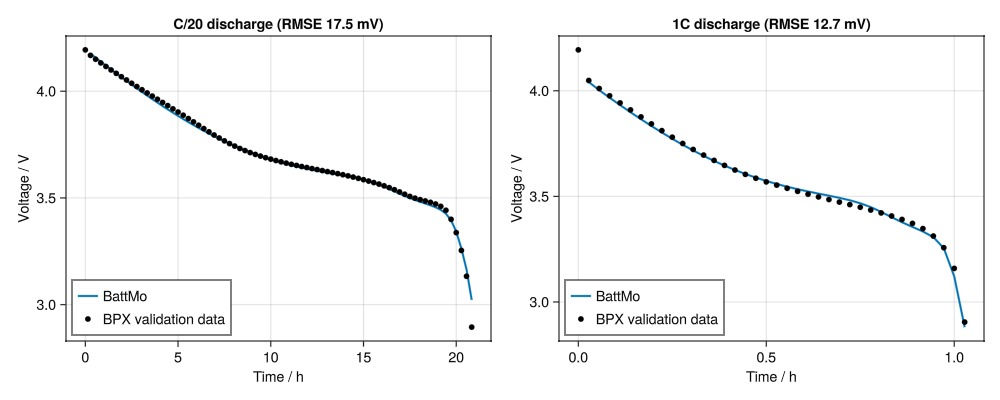
The simulations reproduce both validation curves with an RMSE below 20 mV.
Export to BPX
A BattMo parameter set can be written to a BPX file with write_bpx. The voltage cut-offs and the initial state are taken from the cycling protocol. The export is validated against the BPX schema and reports parameters that BPX cannot represent.
exported_file_path = joinpath(mktempdir(), "nmc_pouch_cell_BPX.json")
write_bpx(exported_file_path, cell_parameters; cycling_protocol)
Dict{String, Any} with 3 entries:
"Parameterisation" => {…
"State" => {…
"Header" => {…The exported file can be loaded again and gives the same parameters.
reloaded = load_cell_parameters(; from_bpx_file_path = exported_file_path)
println("Electrode area after the round trip: ", reloaded["Cell"]["ElectrodeGeometricSurfaceArea"], " m²")
┌ Warning: BPX import: the result differs from the input or needs attention. See the "BPX parameter sets" page of the BattMo documentation.
│
│ Inconsistencies within the BPX data:
│ - Parameterisation: the maximum voltage given by the OCPs at the stoichiometry limits (4.2018 V) is above the upper voltage cut-off (4.2 V).
│
│ Differences between the BPX and BattMo models:
│ - Thermal model: BPX uses a lumped heat balance for the whole cell, with heat capacity density × specific heat capacity × cell volume (cell volume 7.3434152e-5 m3) and cooling by the heat transfer coefficient over the external surface area (0.0379 m2). BattMo resolves the temperature in the simulated electrode stack only (volume 7.343e-5 m3, 100.0 % of the cell volume) and cools it through the faces of the simulation grid with Cell → SurfaceHeatTransferCoefficient. The cell volume, the external surface area and the heat transfer coefficient are not used, so thermal simulations do not reproduce BPX. Isothermal simulations are unaffected.
└ @ BattMo.BPX ~/work/BattMo.jl/BattMo.jl/src/input/bpx.jl:133
┌ Info: BPX import: details of the conversion.
│
│ Approximations made in the conversion:
│ - BPX only gives a lumped cell density (1846.9999999999998 kg.m-3), which is used as the density of every component (active material, inactive solid, electrolyte and separator). The simulated electrochemistry is unaffected; masses and gravimetric quantities are approximate.
│ - Parameterisation → Negative electrode: BPX describes the active material only (volume fraction surface area × radius / 3 = 0.686 of the coating). The rest of the solid (0.06 of the coating) is lumped into the binder; the conductive additive has zero mass.
│ - Parameterisation → Positive electrode: BPX describes the active material only (volume fraction surface area × radius / 3 = 0.6625 of the coating). The rest of the solid (0.06 of the coating) is lumped into the binder; the conductive additive has zero mass.
│ - Electrolyte: BattMo has no activation energies for the electrolyte, so the BPX activation energies are folded into the conductivity and diffusivity functions as Arrhenius factors exp(Ea / R (1 / 298.15 - 1 / T)). This is exact.
│
│ Parameters without a counterpart (not converted):
│ - Parameterisation → Cell → Volume [m3]: volume of the BPX lumped thermal model (see the thermal model difference).
│
│ Operating conditions, which belong to the BattMo CyclingProtocol (load them with `load_cycling_protocol(; from_bpx_file_path)`):
│ - Lower voltage cut-off [V] = 2.7 → CyclingProtocol["LowerVoltageLimit"]
│ - Upper voltage cut-off [V] = 4.2 → CyclingProtocol["UpperVoltageLimit"]
│ - Initial state-of-charge = 1 → CyclingProtocol["InitialStateOfCharge"]
│ - Initial temperature [K] = 298.15 → CyclingProtocol["InitialTemperature"]
│ - Ambient temperature [K] = 298.15 → CyclingProtocol["AmbientTemperature"]
│
│ Notes:
└ - Cell → Case = "Pouch" (cell format) was inferred from the header title or description, since BPX does not specify it. Pass `cell_case` to override it.
Electrode area after the round trip: 0.016808 m²Example on GitHub
If you would like to run this example yourself, it can be downloaded from the BattMo.jl GitHub repository as a script.
This page was generated using Literate.jl.