Validation of Arrhenius temperature dependence implementation in BattMo.jl
This notebook validates the Arrhenius temperature dependence implemented in BattMo.jl for the reaction rate constant k and the solid‑phase diffusion coefficient D, for both the negative and positive electrodes.
BattMo applies an Arrhenius law of the (shifted) form: ln Y(T) = ln Y(T_ref) - (Ea/R) * (1/T - 1/T_ref) so that ln Y varies linearly with (1/T - 1/T_ref) with slope = -Ea/R and intercept ln Y(T_ref).
Steps:
Run simulations at multiple temperatures (0–40 °C) + one at T_ref
Extract k and D at the first output time
Fit ln(Y) vs (1/T - 1/T_ref)
Compare fitted slope to theoretical -Ea/R
Plot data, fitted lines, and theory lines (anchored at ln Y_ref)
using BattMo
using GLMakie
using Statistics
Load model with Arrhenius temperature dependence
cell_parameters = load_cell_parameters(; from_default_set = "chen_2020")
cycling_protocol = load_cycling_protocol(; from_default_set = "cc_discharge")
model_settings = load_model_settings(; from_default_set = "p2d")

model_settings["TemperatureDependence"] = "Arrhenius"
model = LithiumIonBattery(; model_settings)

temps_C = 0:10:40   # 0,10,20,30,40 °C

T_ref = 298.15298.15Activation energies from parameter set (assumed in J/mol)
Ea_ne_R = cell_parameters["NegativeElectrode"]["ActiveMaterial"]["ActivationEnergyOfReaction"]
Ea_ne_D = cell_parameters["NegativeElectrode"]["ActiveMaterial"]["ActivationEnergyOfDiffusion"]
Ea_pe_R = cell_parameters["PositiveElectrode"]["ActiveMaterial"]["ActivationEnergyOfReaction"]
Ea_pe_D = cell_parameters["PositiveElectrode"]["ActiveMaterial"]["ActivationEnergyOfDiffusion"]5000Run simulations and extract values
T = Float64[]     # K
kvals_ne = Float64[]     # reaction rate (NE)
Dvals_ne = Float64[]     # diffusion (NE)
kvals_pe = Float64[]     # reaction rate (PE)
Dvals_pe = Float64[]     # diffusion (PE)

for TC in temps_C
    p = deepcopy(cycling_protocol)
    p["InitialTemperature"] = TC + 273.15
    sim = Simulation(model, cell_parameters, p)
    out = solve(sim; info_level = -1)

    k_ne = out.states["NegativeElectrode"]["ActiveMaterial"]["ReactionRateConstant"][1, :]
    d_ne = out.states["NegativeElectrode"]["ActiveMaterial"]["DiffusionCoefficient"][1, :]
    k_pe = out.states["PositiveElectrode"]["ActiveMaterial"]["ReactionRateConstant"][1, :]
    d_pe = out.states["PositiveElectrode"]["ActiveMaterial"]["DiffusionCoefficient"][1, :]

    push!(kvals_ne, mean(filter(!isnan, collect(k_ne))))
    push!(Dvals_ne, mean(filter(!isnan, collect(d_ne))))
    push!(kvals_pe, mean(filter(!isnan, collect(k_pe))))
    push!(Dvals_pe, mean(filter(!isnan, collect(d_pe))))

    push!(T, TC + 273.15)
end
✔️ Validation of CellParameters passed: No issues found.
──────────────────────────────────────────────────
✔️ Validation of CyclingProtocol passed: No issues found.
──────────────────────────────────────────────────
✔️ Validation of SimulationSettings passed: No issues found.
──────────────────────────────────────────────────
✔️ Validation of SolverSettings passed: No issues found.
──────────────────────────────────────────────────
✔️ Validation of CellParameters passed: No issues found.
──────────────────────────────────────────────────
✔️ Validation of CyclingProtocol passed: No issues found.
──────────────────────────────────────────────────
✔️ Validation of SimulationSettings passed: No issues found.
──────────────────────────────────────────────────
✔️ Validation of SolverSettings passed: No issues found.
──────────────────────────────────────────────────Also run once at the reference temperature to anchor the theoretical lines at ln(Y_ref)
p_ref = deepcopy(cycling_protocol)
p_ref["InitialTemperature"] = T_ref
sim = Simulation(model, cell_parameters, p_ref)
out_ref = solve(sim; info_level = -1);

k_ne_ref = out_ref.states["NegativeElectrode"]["ActiveMaterial"]["ReactionRateConstant"][1, :]
d_ne_ref = out_ref.states["NegativeElectrode"]["ActiveMaterial"]["DiffusionCoefficient"][1, :]
k_pe_ref = out_ref.states["PositiveElectrode"]["ActiveMaterial"]["ReactionRateConstant"][1, :]
d_pe_ref = out_ref.states["PositiveElectrode"]["ActiveMaterial"]["DiffusionCoefficient"][1, :]

k_ne_ref_val = mean(filter(!isnan, collect(k_ne_ref)))
d_ne_ref_val = mean(filter(!isnan, collect(d_ne_ref)))
k_pe_ref_val = mean(filter(!isnan, collect(k_pe_ref)))
d_pe_ref_val = mean(filter(!isnan, collect(d_pe_ref)))4.000000000000001e-15Fit ln(k) and ln(D) vs (1/T - 1/T_ref)
function linfit(x, y)
    x̄ = mean(x)
    ȳ = mean(y)
    b = sum((x .- x̄) .* (y .- ȳ)) / sum((x .- x̄) .^ 2)
    a = ȳ - b * x̄
    return a, b
end

R = Constants().R
x_ref = (1.0 ./ T) .- (1.0 / T_ref)

a_k_ne, b_k_ne = linfit(x_ref, log.(kvals_ne))
a_D_ne, b_D_ne = linfit(x_ref, log.(Dvals_ne))
a_k_pe, b_k_pe = linfit(x_ref, log.(kvals_pe))
a_D_pe, b_D_pe = linfit(x_ref, log.(Dvals_pe))

slope_fit_k_ne = b_k_ne
slope_fit_D_ne = b_D_ne
slope_fit_k_pe = b_k_pe
slope_fit_D_pe = b_D_pe-601.3617752136347Theoretical slopes: -Ea/R
slope_theory_k_ne = -Ea_ne_R / R
slope_theory_D_ne = -Ea_ne_D / R
slope_theory_k_pe = -Ea_pe_R / R
slope_theory_D_pe = -Ea_pe_D / R

ln_k_ne_ref = log(k_ne_ref_val)
ln_D_ne_ref = log(d_ne_ref_val)
ln_k_pe_ref = log(k_pe_ref_val)
ln_D_pe_ref = log(d_pe_ref_val)-33.1524820337908Plot the simulation data, fitted lines, and theoretical lines (shifted-x)
fig1 = Figure(size = (1200, 900))

xs = range(minimum(x_ref), maximum(x_ref), length = 100)


ax1 = Axis(
    fig1[1, 1],
    title = "Arrhenius Validation (with T_ref): NE reaction rate constant k",
    xlabel = "1/T - 1/T_ref (1/K)", ylabel = "ln(k)",
)
scatter!(ax1, x_ref, log.(kvals_ne), color = :blue, label = "Simulation data")
lines!(
    ax1, xs, a_k_ne .+ b_k_ne .* xs, color = :blue,
    label = "Fit slope = $(round(slope_fit_k_ne, digits = 4))",
)
lines!(
    ax1, xs, ln_k_ne_ref .+ slope_theory_k_ne .* xs,
    color = :black, linestyle = :dash,
    label = "Theory slope = $(round(slope_theory_k_ne, digits = 4))",
)
axislegend(ax1, position = :rb)

ax2 = Axis(
    fig1[1, 2],
    title = "Arrhenius Validation (with T_ref): PE reaction rate constant k",
    xlabel = "1/T - 1/T_ref (1/K)", ylabel = "ln(k)",
)
scatter!(ax2, x_ref, log.(copy(kvals_pe)), color = :blue, label = "Simulation data")
lines!(
    ax2, xs, a_k_pe .+ b_k_pe .* xs, color = :blue,
    label = "Fit slope = $(round(slope_fit_k_pe, digits = 4))",
)
lines!(
    ax2, xs, ln_k_pe_ref .+ slope_theory_k_pe .* xs,
    color = :black, linestyle = :dash,
    label = "Theory slope = $(round(slope_theory_k_pe, digits = 4))",
)
axislegend(ax2, position = :rb)

ax3 = Axis(
    fig1[2, 1],
    title = "Arrhenius Validation (with T_ref): NE diffusion coefficient D",
    xlabel = "1/T - 1/T_ref (1/K)", ylabel = "ln(D)",
)
scatter!(ax3, x_ref, log.(Dvals_ne), color = :red, label = "Simulation data")
lines!(
    ax3, xs, a_D_ne .+ b_D_ne .* xs, color = :red,
    label = "Fit slope = $(round(slope_fit_D_ne, digits = 4))",
)
lines!(
    ax3, xs, ln_D_ne_ref .+ slope_theory_D_ne .* xs,
    color = :black, linestyle = :dash,
    label = "Theory slope = $(round(slope_theory_D_ne, digits = 4))",
)
axislegend(ax3, position = :rb)

ax4 = Axis(
    fig1[2, 2],
    title = "Arrhenius Validation (with T_ref): PE diffusion coefficient D",
    xlabel = "1/T - 1/T_ref (1/K)", ylabel = "ln(D)",
)
scatter!(ax4, x_ref, log.(Dvals_pe), color = :red, label = "Simulation data")
lines!(
    ax4, xs, a_D_pe .+ b_D_pe .* xs, color = :red,
    label = "Fit slope = $(round(slope_fit_D_pe, digits = 4))",
)
lines!(
    ax4, xs, ln_D_pe_ref .+ slope_theory_D_pe .* xs,
    color = :black, linestyle = :dash,
    label = "Theory slope = $(round(slope_theory_D_pe, digits = 4))",
)
axislegend(ax4, position = :rb)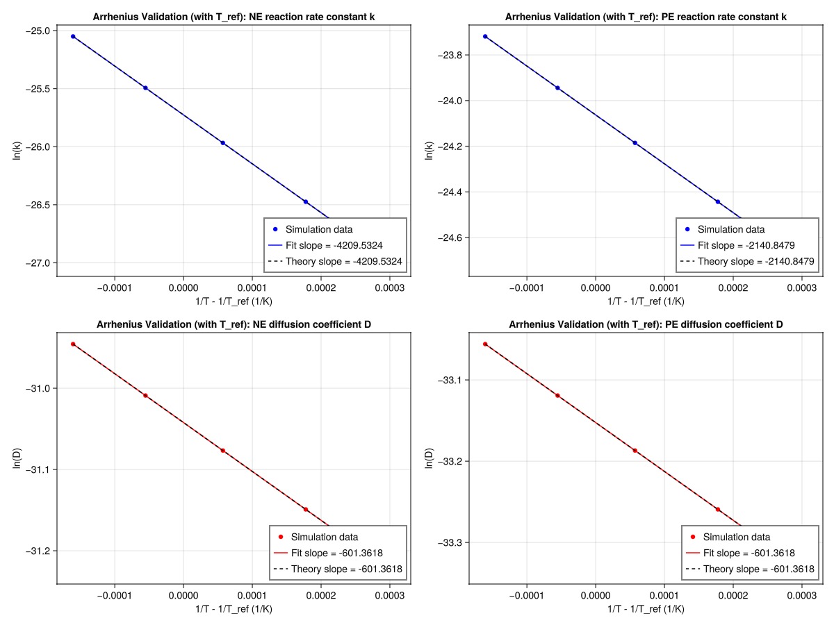
From te results, we can see that the log(k) and log(D) values from the simulations have a linear relationship with (1/T - 1/T_ref) and that the fitted lines closely follow the theoretical lines, which are anchored at the reference temperature point. We can also see that the fitted slopes (from the simulation data) closely match the theoretical slopes (-Ea/R), validating the Arrhenius temperature dependence implementation.
Example on GitHub
If you would like to run this example yourself, it can be downloaded from the BattMo.jl GitHub repository as a script.
This page was generated using Literate.jl.