Handling cycling protocols

In this tutorial, we demonstrate functionality to handle cycling protcols. We will illustrate the effect that the DRate has on battery performance during discharge, using a constant-current (CC) discharge protocol.

Load required packages and data

We start by loading the necessary parameters sets and instantiating a model. For the cyling protocol, we'll start from the default constant current discharge protocol.

using BattMo, GLMakie, Printf

Load cell and model setup

cell_parameters = load_cell_parameters(; from_default_set = "chen_2020")
cc_discharge_protocol = load_cycling_protocol(; from_default_set = "cc_discharge")

{
    "DRate" => 0.5
    "Protocol" => "CC"
    "LowerVoltageLimit" => 2.4
    "Metadata" =>     {
        "Description" => "Parameter set for a constant current discharging protocol."
        "Title" => "cc_discharge"
    }
    "TotalNumberOfCycles" => 0
    "InitialControl" => "discharging"
    "UpperVoltageLimit" => 4.1
    "InitialStateOfCharge" => 0.99
}

Load default model

model = LithiumIonBattery()

LithiumIonBattery("Setup object for a P2D lithium-ion model", {
    "PotentialFlowDiscretization" => "GeneralAD"
    "ModelFramework" => "P2D"
    "Metadata" =>     {
        "Description" => "Default model settings for a P2D simulation including a current ramp up, excluding current collectors and SEI effects."
        "Title" => "p2d"
    }
    "RampUp" => "Sinusoidal"
    "TransportInSolid" => "FullDiffusion"
    "ButlerVolmer" => "Standard"
}, true, #undef)

Handle, access and edit cycling protocols

We manipulate a cycling protocol in the same was as we do cell parameters in the previous tutorial. To list all outermost keys:

keys(cc_discharge_protocol)

KeySet for a Dict{String, Any} with 8 entries. Keys:
  "DRate"
  "Protocol"
  "LowerVoltageLimit"
  "Metadata"
  "TotalNumberOfCycles"
  "InitialControl"
  "UpperVoltageLimit"
  "InitialStateOfCharge"

Show all keys and values

cc_discharge_protocol.all

Dict{String, Any} with 8 entries:
  "DRate"                => 0.5
  "Protocol"             => "CC"
  "LowerVoltageLimit"    => 2.4
  "Metadata"             => {…
  "TotalNumberOfCycles"  => 0
  "InitialControl"       => "discharging"
  "UpperVoltageLimit"    => 4.1
  "InitialStateOfCharge" => 0.99

Search for a specific parameter

search_parameter(cc_discharge_protocol, "rate")

Parameters
------------------
[ "DRate" ] => 0.5

Access a specific parameter

cc_discharge_protocol["DRate"]

0.5

Change protocol parameters as dicitonaries

cc_discharge_protocol["DRate"] = 2.0

2.0

Compare cell performance across DRates

Lets now do something more fun. Since we can edit scalar valued parameters as we edit dictionaries, we can loop through different DRates and run a simulation for each. We can then compare the cell voltage profiles for each DRate.

Let’s define the range of C-rates to explore:

d_rates = [0.2, 0.5, 1.0, 2.0]

4-element Vector{Float64}:
 0.2
 0.5
 1.0
 2.0

Now loop through these values, update the protocol, and store the results:

outputs = []

for d_rate in d_rates
    protocol = deepcopy(cc_discharge_protocol)
    protocol["DRate"] = d_rate

    sim = Simulation(model, cell_parameters, protocol)
    output = solve(sim; info_level = -1)
    push!(outputs, (d_rate = d_rate, output = output))
end

✔️ Validation of CellParameters passed: No issues found.
──────────────────────────────────────────────────
✔️ Validation of CyclingProtocol passed: No issues found.
──────────────────────────────────────────────────
✔️ Validation of SimulationSettings passed: No issues found.
──────────────────────────────────────────────────
✔️ Validation of SolverSettings passed: No issues found.
──────────────────────────────────────────────────
✔️ Validation of CellParameters passed: No issues found.
──────────────────────────────────────────────────
✔️ Validation of CyclingProtocol passed: No issues found.
──────────────────────────────────────────────────
✔️ Validation of SimulationSettings passed: No issues found.
──────────────────────────────────────────────────
✔️ Validation of SolverSettings passed: No issues found.
──────────────────────────────────────────────────
✔️ Validation of CellParameters passed: No issues found.
──────────────────────────────────────────────────
✔️ Validation of CyclingProtocol passed: No issues found.
──────────────────────────────────────────────────
✔️ Validation of SimulationSettings passed: No issues found.
──────────────────────────────────────────────────
✔️ Validation of SolverSettings passed: No issues found.
──────────────────────────────────────────────────
✔️ Validation of CellParameters passed: No issues found.
──────────────────────────────────────────────────
✔️ Validation of CyclingProtocol passed: No issues found.
──────────────────────────────────────────────────
✔️ Validation of SimulationSettings passed: No issues found.
──────────────────────────────────────────────────
✔️ Validation of SolverSettings passed: No issues found.
──────────────────────────────────────────────────

Analyze Voltage and Capacity

We'll extract the voltage vs. time and delivered capacity for each C-rate:

fig = Figure(size = (1000, 400))
ax1 = Axis(fig[1, 1], title = "Voltage vs Time", xlabel = "Time / s", ylabel = "Voltage / V")

for result in outputs

    t = result.output.time_series["Time"]
    E = result.output.time_series["Voltage"]
    I = result.output.time_series["Current"]

    label_str = @sprintf("%.1fC", result.d_rate)
    lines!(ax1, t, E, label = label_str)

end

fig[1, 3] = Legend(fig, ax1, "C-rates", framevisible = false)
fig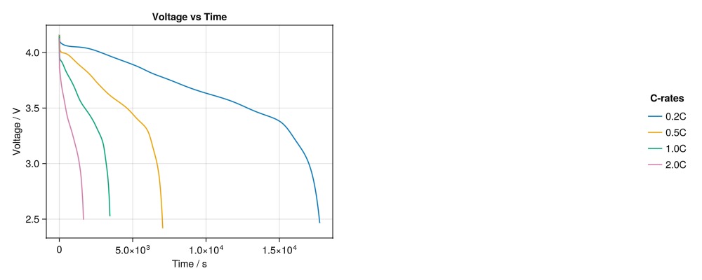

We see this cell has poor power capabilities since its capacity decreases quite rapidly with DRate.

Example on GitHub

If you would like to run this example yourself, it can be downloaded from the BattMo.jl GitHub repository as a script.

---

This page was generated using Literate.jl.