3D pouch cell geometry and plotting

This example shows how to:

• modify the pouch-cell geometry before running a simulation

• inspect the generated 3D grids and tab locations

• plot different output fields on the component meshes

• launch the interactive 3D output viewer

using BattMo, GLMakie, Jutul

Load default parameter sets

cell_parameters = load_cell_parameters(; from_default_set = "xu_2015")
cycling_protocol = load_cycling_protocol(; from_default_set = "cc_discharge")
model_settings = load_model_settings(; from_default_set = "p4d_pouch")
simulation_settings = load_simulation_settings(; from_default_set = "p4d_pouch")

Modify the pouch geometry

The pouch geometry is controlled by a combination of cell parameters and simulation settings. Some useful quantities to experiment with are:

• TabsOnSameSide

• TabPositionFraction

• TabWidth and TabLength

• current collector thickness

• in-plane grid resolution

cycling_protocol["DRate"] = 1

1

Move the tabs so that the current collectors connect at different x-positions.

cell_parameters["NegativeElectrode"]["CurrentCollector"]["TabPositionFraction"] = 0.20
cell_parameters["PositiveElectrode"]["CurrentCollector"]["TabPositionFraction"] = 0.80

0.8

Toggle whether the tabs are on the same side of the pouch or opposite sides.

cell_parameters["Cell"]["TabsOnSameSide"] = true

true

Increase the tab dimensions to make them easier to see in the geometry plots.

cell_parameters["Cell"]["TabWidth"] = 20e-3
cell_parameters["Cell"]["TabLength"] = 12e-3

0.012

Thicker current collectors are also easier to visualize.

cell_parameters["NegativeElectrode"]["CurrentCollector"]["Thickness"] = 18e-6
cell_parameters["PositiveElectrode"]["CurrentCollector"]["Thickness"] = 20e-6

2.0e-5

A slightly coarser in-plane grid keeps the example fairly quick to set up.

simulation_settings["ElectrodeWidthGridPoints"] = 12
simulation_settings["ElectrodeLengthGridPoints"] = 8

Create the simulation object

model = LithiumIonBattery(; model_settings)
sim = Simulation(model, cell_parameters, cycling_protocol; simulation_settings)

grids = sim.grids
couplings = sim.couplings

components = ["NegativeElectrode", "PositiveElectrode", "NegativeCurrentCollector", "PositiveCurrentCollector"]
colors = [:gray, :green, :dodgerblue, :black]

✔️ Validation of ModelSettings passed: No issues found.
──────────────────────────────────────────────────
✔️ Validation of CellParameters passed: No issues found.
──────────────────────────────────────────────────
✔️ Validation of CyclingProtocol passed: No issues found.
──────────────────────────────────────────────────
✔️ Validation of SimulationSettings passed: No issues found.
──────────────────────────────────────────────────

Plot the component meshes

for (i, component) in enumerate(components)
	if i == 1
		global fig_mesh, ax_mesh = plot_mesh(grids[component];
			color = colors[i],
			label = component)
	else
		plot_mesh!(ax_mesh, grids[component];
			color = colors[i],
			label = component)
	end
end

Legend(fig_mesh[1, 2], [PolyElement(color = c) for c in colors], components)
ax_mesh.aspect = :data
ax_mesh.azimuth[] = 5.2
ax_mesh.elevation[] = 0.45
fig_mesh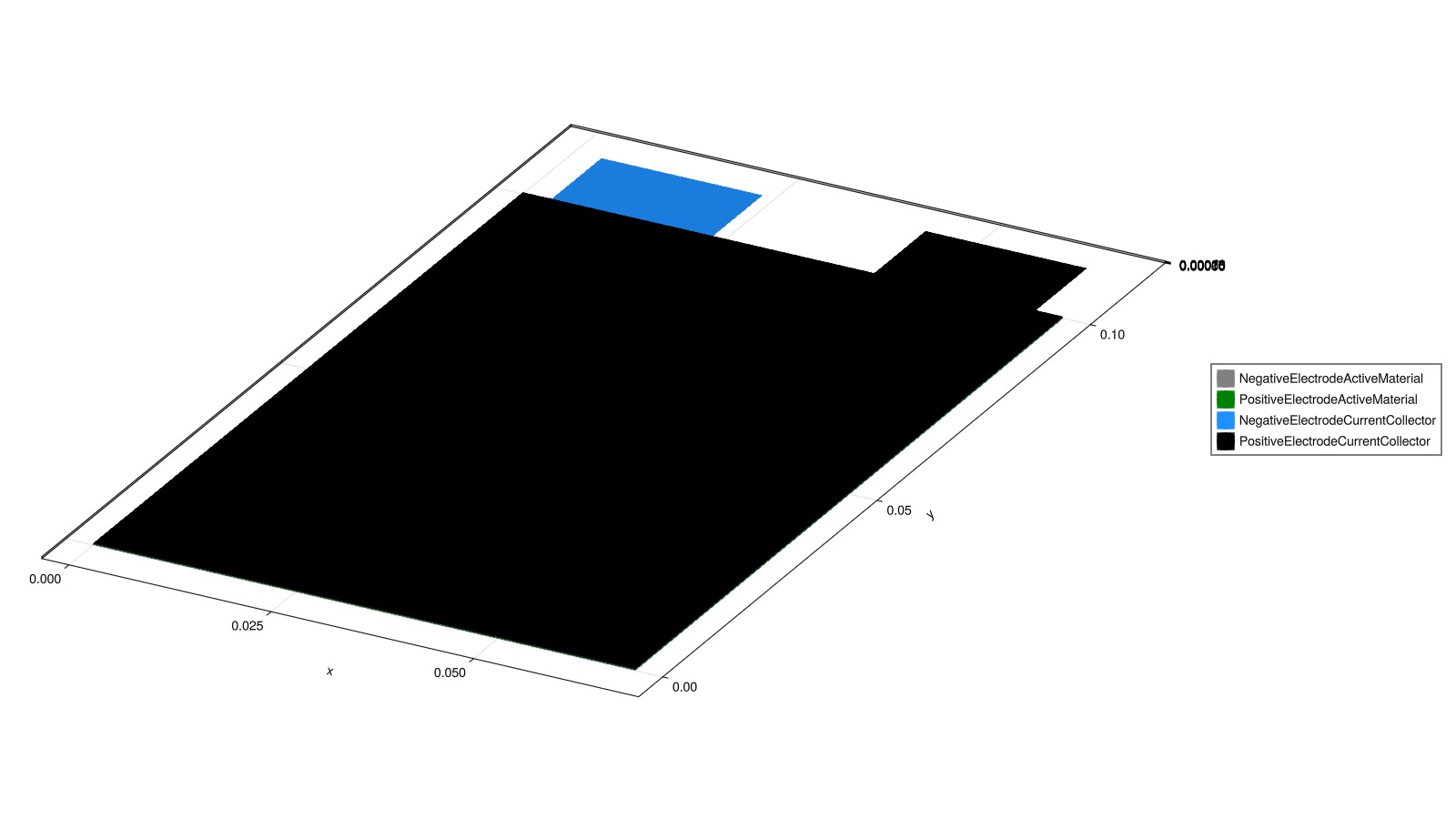

Plot mesh edges and highlight the tabs

The external couplings on the current collectors correspond to the tab faces. We plot those in red on top of the mesh edges.

for (i, component) in enumerate(components)
	if i == 1
		global fig_edges, ax_edges = plot_mesh_edges(grids[component];
			color = colors[i],
			label = component)
	else
		plot_mesh_edges!(ax_edges, grids[component];
			color = colors[i],
			label = component)
	end
end

for component in ["NegativeCurrentCollector", "PositiveCurrentCollector"]
	plot_mesh!(ax_edges, grids[component];
		boundaryfaces = couplings[component]["External"]["boundaryfaces"],
		color = :red)
end

Legend(fig_edges[1, 2], [PolyElement(color = c) for c in colors], components)
ax_edges.aspect = :data
ax_edges.azimuth[] = 5.2
ax_edges.elevation[] = 0.45
fig_edges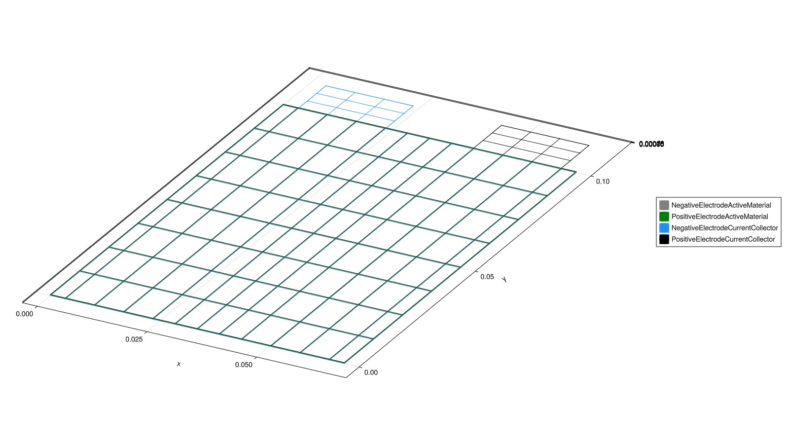

Run the simulation

output = solve(sim)

✔️ Validation of SolverSettings passed: No issues found.
──────────────────────────────────────────────────
Jutul: Simulating 1 hour, 6 minutes as 84 report steps
╭────────────────┬──────────┬──────────────┬──────────╮
│ Iteration type │ Avg/step │ Avg/ministep │    Total │
│                │ 72 steps │ 72 ministeps │ (wasted) │
├────────────────┼──────────┼──────────────┼──────────┤
│ Newton         │  2.59722 │      2.59722 │  187 (0) │
│ Linearization  │  3.59722 │      3.59722 │  259 (0) │
│ Linear solver  │  2.59722 │      2.59722 │  187 (0) │
│ Precond apply  │      0.0 │          0.0 │    0 (0) │
╰────────────────┴──────────┴──────────────┴──────────╯
╭───────────────┬──────────┬────────────┬─────────╮
│ Timing type   │     Each │   Relative │   Total │
│               │       ms │ Percentage │       s │
├───────────────┼──────────┼────────────┼─────────┤
│ Properties    │   5.3875 │     1.84 % │  1.0075 │
│ Equations     │ 136.1449 │    64.47 % │ 35.2615 │
│ Assembly      │   4.6174 │     2.19 % │  1.1959 │
│ Linear solve  │  70.0391 │    23.95 % │ 13.0973 │
│ Linear setup  │   0.0000 │     0.00 % │  0.0000 │
│ Precond apply │   0.0000 │     0.00 % │  0.0000 │
│ Update        │   1.9130 │     0.65 % │  0.3577 │
│ Convergence   │   3.9750 │     1.88 % │  1.0295 │
│ Input/Output  │   1.3556 │     0.18 % │  0.0976 │
│ Other         │  14.1620 │     4.84 % │  2.6483 │
├───────────────┼──────────┼────────────┼─────────┤
│ Total         │ 292.4885 │   100.00 % │ 54.6954 │
╰───────────────┴──────────┴────────────┴─────────╯

Plot different fields on the 3D meshes

The BattMo output now stores component-wise positions, so the state fields can be plotted directly against the corresponding component geometry.

Potential in the negative current collector

fig_phi, ax_phi = plot_cell_data(
	output.states["NegativeElectrode"]["CurrentCollector"]["Position"],
	output.states["NegativeElectrode"]["CurrentCollector"]["Potential"][end, :];
	colormap = :viridis,
)
ax_phi.aspect = :data
ax_phi.title = "Negative current collector potential"
fig_phi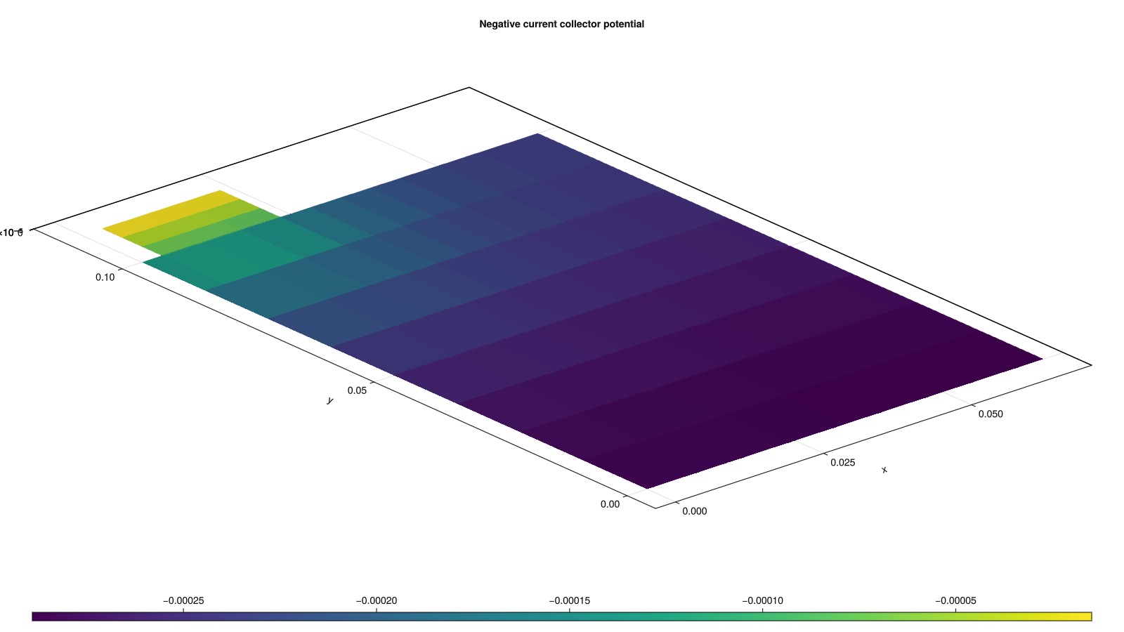

Surface concentration in the positive electrode active material

fig_cs, ax_cs = plot_cell_data(
	output.states["PositiveElectrode"]["ActiveMaterial"]["Position"],
	output.states["PositiveElectrode"]["ActiveMaterial"]["SurfaceConcentration"][end, :];
	colormap = :plasma,
)
ax_cs.aspect = :data
ax_cs.title = "Positive electrode surface concentration"
fig_cs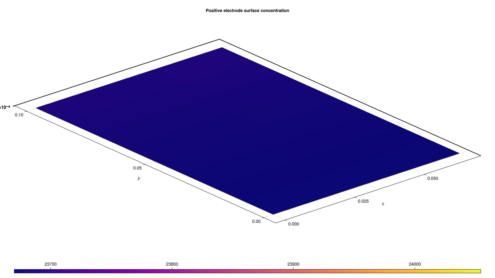

Mesh edges can be overlaid on top of a cell-data plot.

plot_mesh_edges!(ax_cs, output.states["PositiveElectrode"]["ActiveMaterial"]["Position"];
	color = :black,
	linewidth = 0.5)
fig_cs

Double coated electrodes and Multi-layer pouch geometry

We can also create a multi-layer pouch geometry by modifying the Cell parameters. The number of layers is controlled by NumberOfLayersInParallel, and for a single layer simulation we can also choose to have double coated electrodes by setting DoubleCoatedElectrodes to true.

Let's plot the mesh for a double-coated single-layer pouch cell.

cell_parameters["Cell"]["DoubleCoatedElectrodes"] = true

sim = Simulation(model, cell_parameters, cycling_protocol; simulation_settings)
grids = sim.grids
couplings = sim.couplings

for (i, component) in enumerate(components)
	if i == 1
		global fig_edges_d, ax_edges_d = plot_mesh(grids[component];
			color = colors[i],
			label = component)
	else
		plot_mesh!(ax_edges_d, grids[component];
			color = colors[i],
			label = component)
	end
end

for component in ["NegativeCurrentCollector", "PositiveCurrentCollector"]
	plot_mesh!(ax_edges_d, grids[component];
		boundaryfaces = couplings[component]["External"]["boundaryfaces"],
		color = :red)
end

Legend(fig_edges_d[1, 2], [PolyElement(color = c) for c in colors], components)
ax_edges_d.azimuth[] = 5.2
ax_edges_d.elevation[] = 0.45
fig_edges_d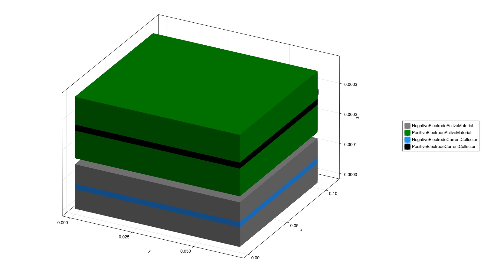

Let's plot the mesh for a multi-layer pouch cell.

cell_parameters["Cell"]["NumberOfLayersInParallel"] = 2

sim = Simulation(model, cell_parameters, cycling_protocol; simulation_settings)
grids = sim.grids
couplings = sim.couplings

for (i, component) in enumerate(components)
	if i == 1
		global fig_edges_m, ax_edges_m = plot_mesh(grids[component];
			color = colors[i],
			label = component)
	else
		plot_mesh!(ax_edges_m, grids[component];
			color = colors[i],
			label = component)
	end
end

for component in ["NegativeCurrentCollector", "PositiveCurrentCollector"]
	plot_mesh!(ax_edges_m, grids[component];
		boundaryfaces = couplings[component]["External"]["boundaryfaces"],
		color = :red)
end

Legend(fig_edges_m[1, 2], [PolyElement(color = c) for c in colors], components)
ax_edges_m.azimuth[] = 5.2
ax_edges_m.elevation[] = 0.45
fig_edges_m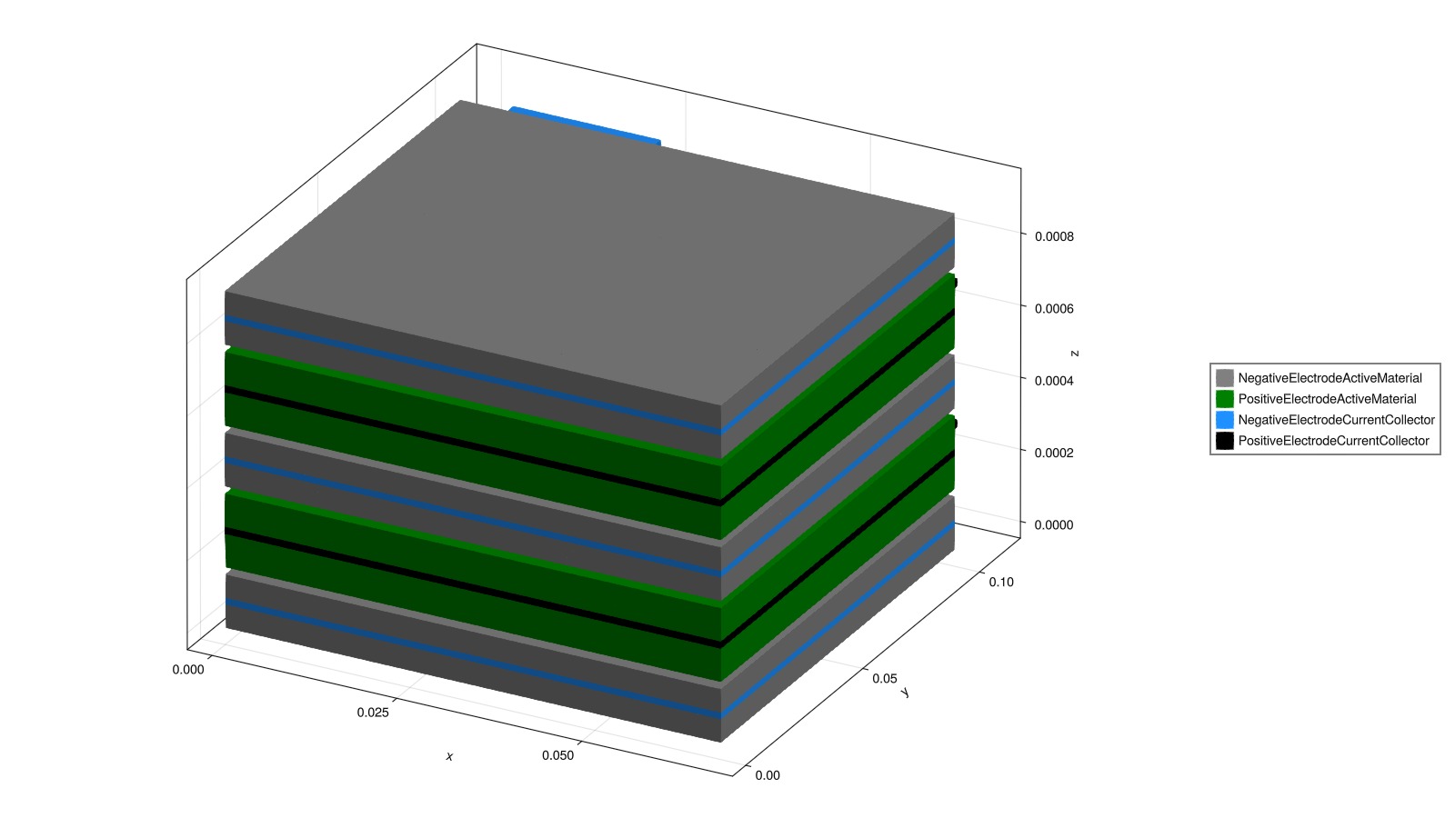

Interactive 3D viewer

We can view the output in an interactive 3D viewer, which allows us to explore the different fields and components in more detail. The viewer can be launched with the plot_interactive_3d function, which takes the simulation output as input.

output = solve(sim)
plot_interactive_3d(output; colormap = :curl)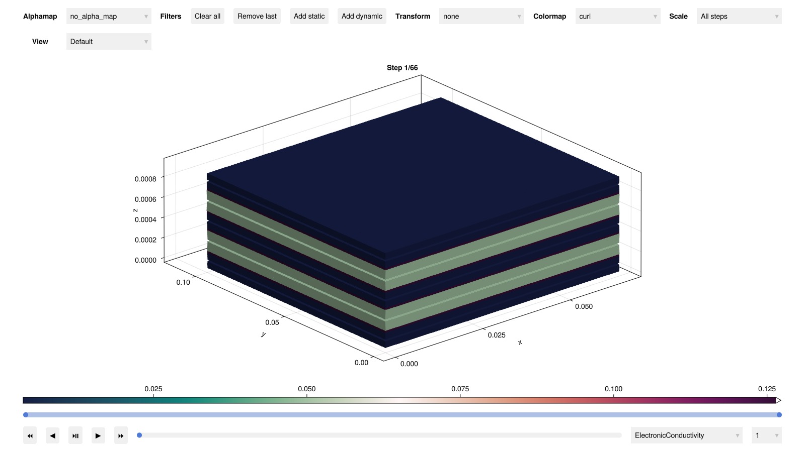

Example on GitHub

If you would like to run this example yourself, it can be downloaded from the BattMo.jl GitHub repository as a script.

---

This page was generated using Literate.jl.