Example with SEI layer
Preparation of the input
julia
using Jutul, BattMo, GLMakieWe use the SEI model presented in [1]. We use the json data given in bolay.json which contains the parameters for the SEI layer.
julia
cell_parameters = load_cell_parameters(; from_default_set = "chen_2020")
cycling_protocol = load_cycling_protocol(; from_default_set = "cccv")
simulation_settings = load_simulation_settings(; from_default_set = "p2d")
We have a look at the SEI related parameters.
julia
interphase_parameters = cell_parameters["NegativeElectrode"]["Interphase"]Dict{String, Any} with 8 entries:
"Description" => "EC-based SEI, from Bolay2022."
"ElectronicDiffusionCoefficient" => 1.6e-12
"InterstitialConcentration" => 0.015
"InitialThickness" => 1.0e-8
"IonicConductivity" => 1.0e-5
"StoichiometricCoefficient" => 2
"InitialPotentialDrop" => 0.5
"MolarVolume" => 9.586e-5We start the simulation and retrieve the result
julia
model = LithiumIonBattery();

model_settings = model.settings
model_settings["SEIModel"] = "Bolay"

cycling_protocol["TotalNumberOfCycles"] = 10

sim = Simulation(model, cell_parameters, cycling_protocol; simulation_settings);

output = solve(sim)

t = output.time_series["Time"]
E = output.time_series["Voltage"]
I = output.time_series["Current"]
✔️ Validation of ModelSettings passed: No issues found.
──────────────────────────────────────────────────
✔️ Validation of CellParameters passed: No issues found.
──────────────────────────────────────────────────
✔️ Validation of CyclingProtocol passed: No issues found.
──────────────────────────────────────────────────
✔️ Validation of SimulationSettings passed: No issues found.
──────────────────────────────────────────────────
✔️ Validation of SolverSettings passed: No issues found.
──────────────────────────────────────────────────
Jutul: Simulating 2 days, 2 hours as 3600 report steps
╭────────────────┬────────────┬────────────────┬──────────────╮
│ Iteration type │ Avg/step │ Avg/ministep │ Total │
│ │ 2630 steps │ 2806 ministeps │ (wasted) │
├────────────────┼────────────┼────────────────┼──────────────┤
│ Newton │ 3.01179 │ 2.82288 │ 7921 (2140) │
│ Linearization │ 4.07871 │ 3.82288 │ 10727 (2247) │
│ Linear solver │ 3.01179 │ 2.82288 │ 7921 (2140) │
│ Precond apply │ 0.0 │ 0.0 │ 0 (0) │
╰────────────────┴────────────┴────────────────┴──────────────╯
╭───────────────┬────────┬────────────┬─────────╮
│ Timing type │ Each │ Relative │ Total │
│ │ ms │ Percentage │ s │
├───────────────┼────────┼────────────┼─────────┤
│ Properties │ 0.0714 │ 5.00 % │ 0.5652 │
│ Equations │ 0.2594 │ 24.61 % │ 2.7823 │
│ Assembly │ 0.1079 │ 10.24 % │ 1.1576 │
│ Linear solve │ 0.6191 │ 43.37 % │ 4.9042 │
│ Linear setup │ 0.0000 │ 0.00 % │ 0.0000 │
│ Precond apply │ 0.0000 │ 0.00 % │ 0.0000 │
│ Update │ 0.0620 │ 4.34 % │ 0.4908 │
│ Convergence │ 0.0959 │ 9.10 % │ 1.0286 │
│ Input/Output │ 0.0308 │ 0.76 % │ 0.0864 │
│ Other │ 0.0369 │ 2.58 % │ 0.2922 │
├───────────────┼────────┼────────────┼─────────┤
│ Total │ 1.4275 │ 100.00 % │ 11.3073 │
╰───────────────┴────────┴────────────┴─────────╯Plot of voltage and current
julia
plot_dashboard(output; plot_type = "simple")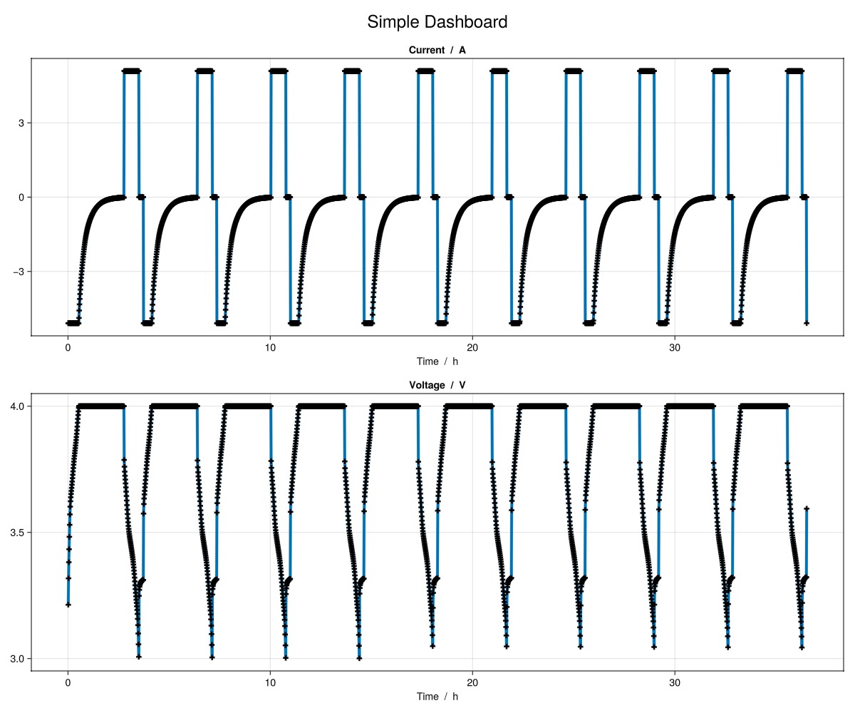
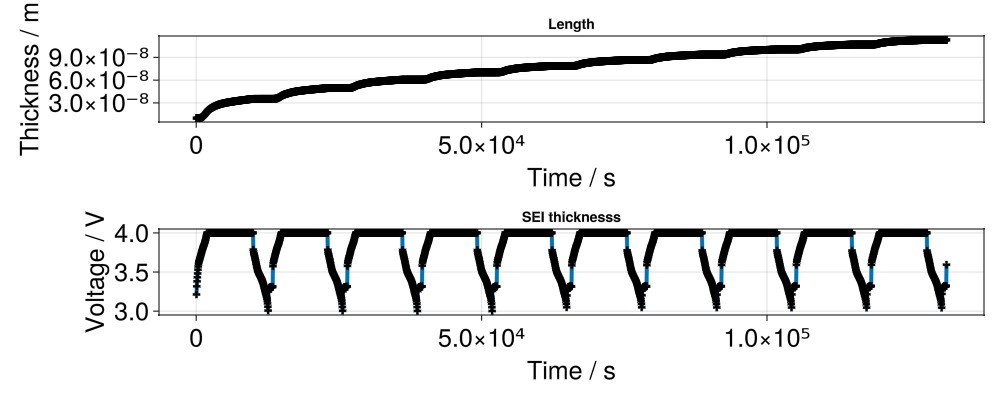
Plot of SEI thickness
We recover the SEI thickness from the state output
julia
seilength_x1 = output.states["NegativeElectrode"]["Interphase"]["Thickness"][:, 1]
seilength_xend = output.states["NegativeElectrode"]["Interphase"]["Thickness"][:, end]

f = Figure(size = (1000, 400))

ax = Axis(
    f[1, 1],
    title = "Length",
    xlabel = "Time / s",
    ylabel = "Thickness / m",
    xlabelsize = 25,
    ylabelsize = 25,
    xticklabelsize = 25,
    yticklabelsize = 25,
)

scatterlines!(
    ax,
    t,
    seilength_x1;
    linewidth = 4,
    markersize = 10,
    marker = :cross,
    markercolor = :black
)

scatterlines!(
    ax,
    t,
    seilength_xend;
    linewidth = 4,
    markersize = 10,
    marker = :cross,
    markercolor = :black
)

ax = Axis(
    f[2, 1],
    title = "SEI thicknesss",
    xlabel = "Time / s",
    ylabel = "Voltage / V",
    xlabelsize = 25,
    ylabelsize = 25,
    xticklabelsize = 25,
    yticklabelsize = 25,
)

scatterlines!(
    ax,
    t,
    E;
    linewidth = 4,
    markersize = 10,
    marker = :cross,
    markercolor = :black
)
Plot of voltage drop
julia
u_x1 = output.states["NegativeElectrode"]["Interphase"]["VoltageDrop"][:, 1]
u_xend = output.states["NegativeElectrode"]["Interphase"]["VoltageDrop"][:, end]

f = Figure(size = (1000, 400))

ax = Axis(
    f[1, 1],
    title = "SEI voltage drop",
    xlabel = "Time / s",
    ylabel = "Voltage / V",
    xlabelsize = 25,
    ylabelsize = 25,
    xticklabelsize = 25,
    yticklabelsize = 25,
)

scatterlines!(
    ax,
    t,
    u_x1;
    linewidth = 4,
    markersize = 10,
    marker = :cross,
    markercolor = :blue,
    label = "xmin"
)

scatterlines!(
    ax,
    t,
    u_xend;
    linewidth = 4,
    markersize = 10,
    marker = :cross,
    markercolor = :black,
    label = "xmax"
)
ScatterLines{Tuple{Vector{Point{2, Float64}}}}Example on GitHub
If you would like to run this example yourself, it can be downloaded from the BattMo.jl GitHub repository as a script.
This page was generated using Literate.jl.