julia
using BattMo, GLMakie

model_settings = load_model_settings(; from_default_set = "p2d")
model_settings["SEIModel"] = "Bolay"
cell_parameters = load_cell_parameters(; from_default_set = "chen_2020")
cycling_protocol = load_cycling_protocol(; from_default_set = "cccv")
simulation_settings = load_simulation_settings(; from_default_set = "p2d")

model = LithiumIonBattery(; model_settings)

cycling_protocol["TotalNumberOfCycles"] = 10

sim = Simulation(model, cell_parameters, cycling_protocol);

output = solve(sim)

print_info(output)

states = output.states
metrics = output.metrics
Dict{String, Any} with 6 entries:
"RoundTripEfficiency" => [78.4004, 88.7218, 88.705, 88.7119, 87.2186, 87.2125…
"DischargeCapacity" => [3.67642, 3.67642, 3.67642, 3.67642, 3.60572, 3.6057…
"DischargeEnergy" => [45365.5, 45331.3, 45304.9, 45282.1, 44492.1, 44474.…
"CycleIndex" => [0, 1, 2, 3, 4, 5, 6, 7, 8, 9]
"ChargeEnergy" => [59002.1, 52099.4, 52079.5, 52049.6, 52034.2, 52017.…
"ChargeCapacity" => [4.23702, 3.6848, 3.68173, 3.67829, 3.67608, 3.67392…Plot a simple pre-defined dashboard
julia
plot_dashboard(output)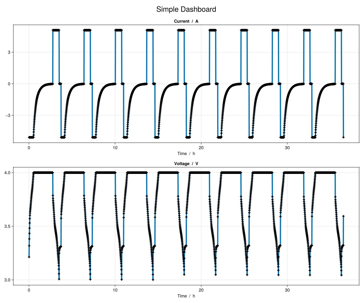
Plot a dashboard with line plots
julia
plot_dashboard(output; plot_type = "line")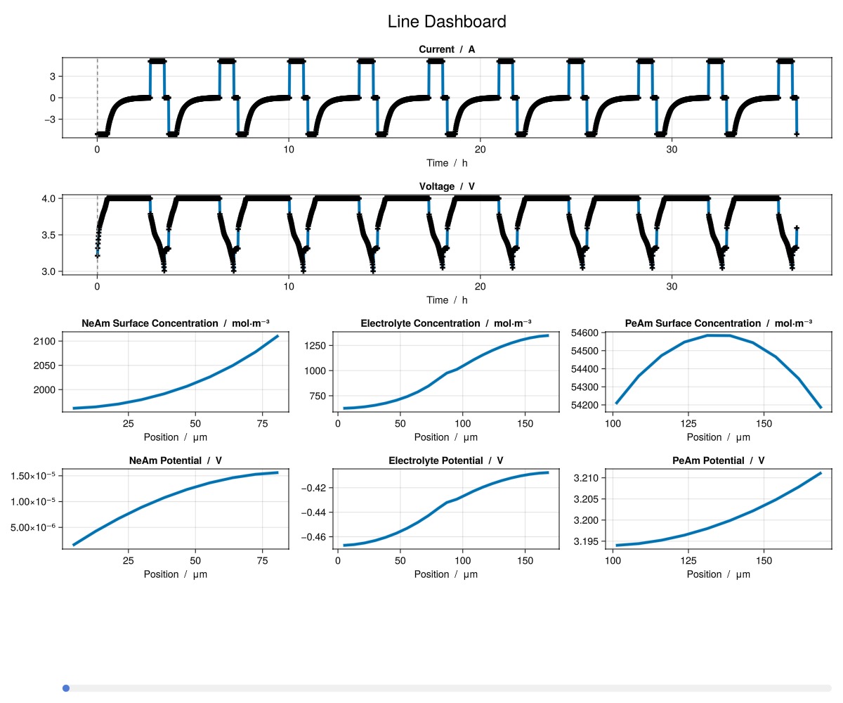
Plot a dashboard with contour plots
julia
plot_dashboard(output; plot_type = "contour")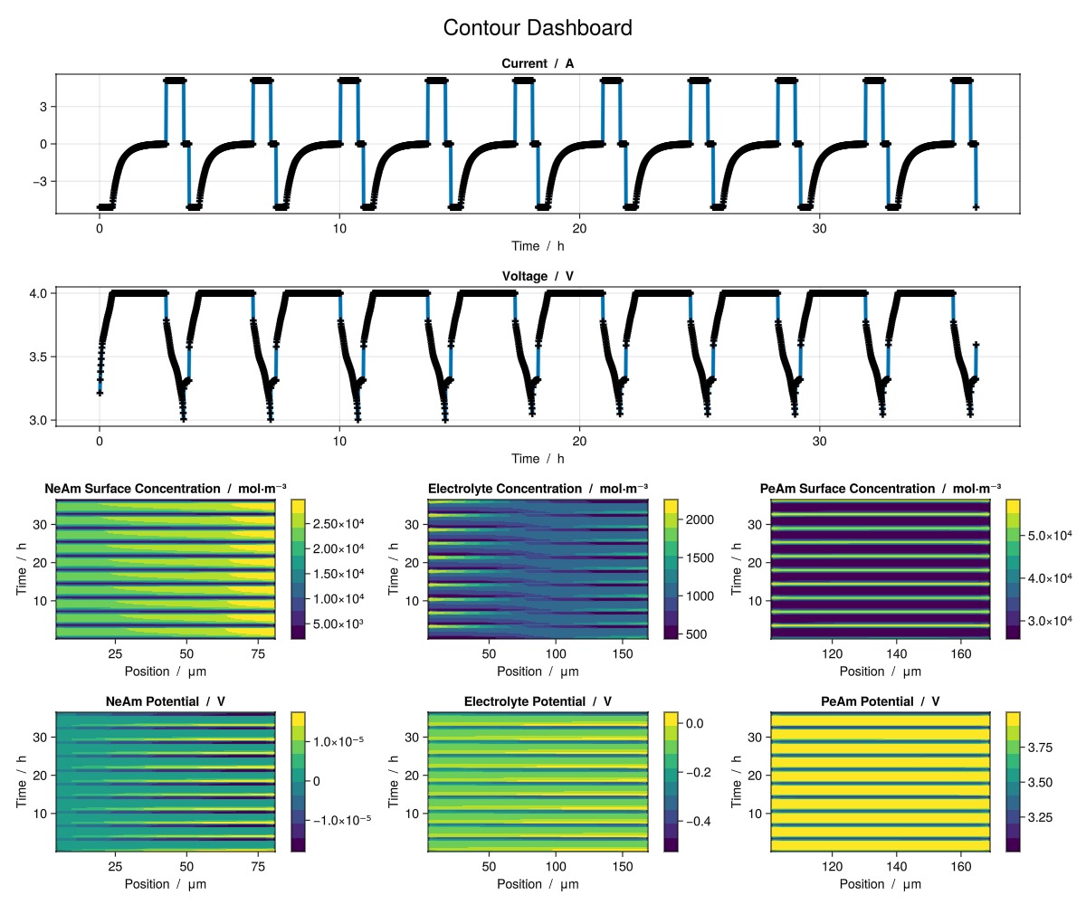
Plot a dashboard with a breakdown of contributions to overpotential
julia
plot_dashboard(output; plot_type = "breakdown")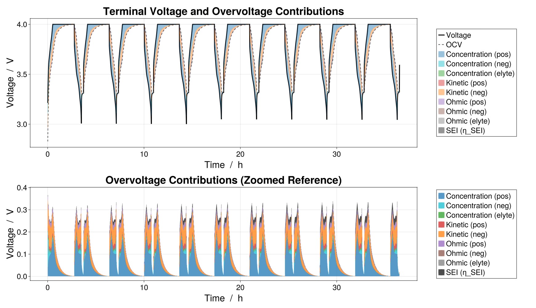
Some simple examples plotting time series quantities using the plot_output function
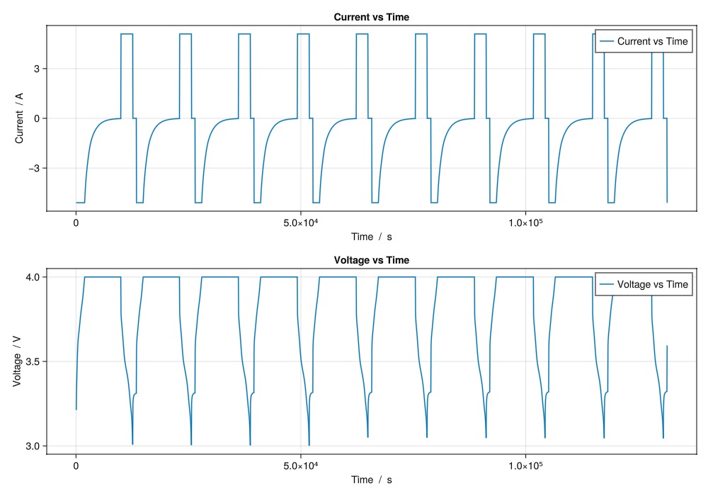
julia
plot_output(
    output,
    [
        "Current vs Time",
        "Voltage vs Time",
    ];
    layout = (2, 1),
)
Some simple examples plotting state quantities using the plot_output function
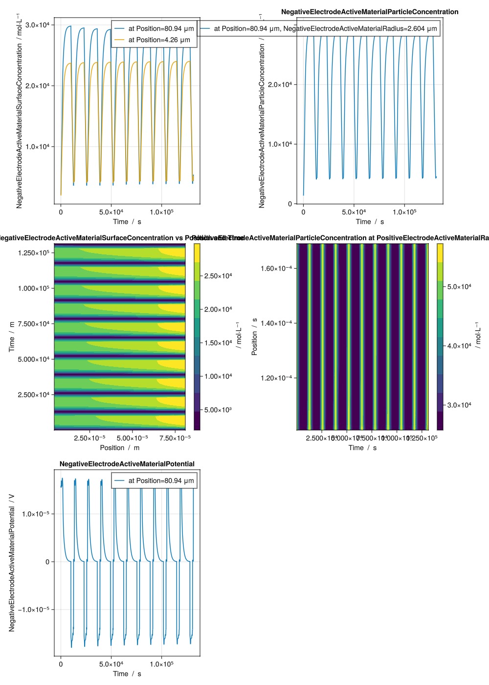
julia
plot_output(
    output,
    [
        ["NegativeElectrodeActiveMaterialSurfaceConcentration vs Time at Position index 10", "NegativeElectrodeActiveMaterialSurfaceConcentration vs Time at Position index 1"],
        "NegativeElectrodeActiveMaterialParticleConcentration vs Time at Position index 10 and NegativeElectrodeActiveMaterialRadius index 5",
        "NegativeElectrodeActiveMaterialSurfaceConcentration vs Position and Time",
        "PositiveElectrodeActiveMaterialParticleConcentration vs Time and Position at PositiveElectrodeActiveMaterialRadius index end",
        "NegativeElectrodeActiveMaterialPotential vs Time at Position index 10",
    ];
    layout = (4, 2),
)
Some simple examples plotting metrics using the plot_output function
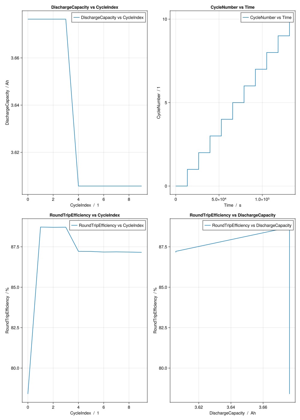
julia
plot_output(
    output,
    [
        "DischargeCapacity vs CycleIndex",
        "CycleNumber vs Time",
        "RoundTripEfficiency vs CycleIndex",
        "RoundTripEfficiency vs DischargeCapacity",
    ];
    layout = (4, 2),
)
Access state data and plot for a specific time step
julia
output_data = output.states;

t = 100 # time step to plot

d1 = output_data["NegativeElectrode"]["ActiveMaterial"]["SurfaceConcentration"][t, :]
d2 = output_data["PositiveElectrode"]["ActiveMaterial"]["SurfaceConcentration"][t, :]
d3 = output_data["Electrolyte"]["Concentration"][t, :]

f = Figure()
ax = Axis(f[1, 1], title = "Concentration at t = $(output_data["Time"][t]) s", xlabel = "Position [m]", ylabel = "Concentration")
l1 = lines!(ax, output_data["Cell"]["Position"], d1, color = :red, linewidth = 2, label = "NeAmSurfaceConcentration")
l2 = lines!(ax, output_data["Cell"]["Position"], d2, color = :blue, linewidth = 2, label = "PeAmSurfaceConcentration")
l3 = lines!(ax, output_data["Cell"]["Position"], d3, color = :green, linewidth = 2, label = "ElectrolyteConcentration")
axislegend(ax)
display(GLMakie.Screen(), f)

g = Figure()
ax2 = Axis(g[1, 1], title = "Active Material Concentration at t = $(output_data["Time"][t]) s", xlabel = "Position", ylabel = "Depth")
hm1 = contourf!(ax2, output_data["Cell"]["Position"], output_data["NegativeElectrode"]["ActiveMaterial"]["Radius"], output_data["NegativeElectrode"]["ActiveMaterial"]["ParticleConcentration"][t, :, :])
hm2 = contourf!(ax2, output_data["Cell"]["Position"], output_data["PositiveElectrode"]["ActiveMaterial"]["Radius"], output_data["PositiveElectrode"]["ActiveMaterial"]["ParticleConcentration"][t, :, :])
Colorbar(g[1, 2], hm1)
display(GLMakie.Screen(), g)GLMakie.Screen(...)Example on GitHub
If you would like to run this example yourself, it can be downloaded from the BattMo.jl GitHub repository as a script.
This page was generated using Literate.jl.